The Hessian Matrix (H-Matrix): Mathematical Foundations, Curvature Analysis & Second-Order Optimization in Data Science

In modern data science and machine learning, nearly every model—from high-dimensional logistic regression to deep neural architectures—is fundamentally framed as an optimization problem:

While first-order optimization algorithms (such as Stochastic Gradient Descent, Adam, and RMSprop) leverage the Gradient Vector ($\nabla \mathcal{L}$) to ascertain the direction of steepest descent, they operate with zero awareness of local landscape curvature.

To understand why gradient descent oscillates violently in ill-conditioned loss valleys (ravines), why high-dimensional non-convex loss surfaces are dominated by saddle points rather than local minima, and how second-order solvers like Newton-Raphson and L-BFGS achieve superlinear and quadratic convergence, we must analyze the Hessian Matrix ($\mathbf{H}$).

1. Formal Mathematical Definition of the Hessian Matrix

Let $f:{\mathbb{R}}^n\to \mathbb{R}$ be a twice continuously differentiable scalar field ($f\in C^2({\mathbb{R}}^n)$).

The gradient of $f$ is the $n\times 1$ column vector of first-order partial derivatives:

The Hessian Matrix ${\mathbf{H}}_f(\mathbf{x})$ (often denoted ${\nabla }^{2}f(\mathbf{x})$) is the $n\times n$ square Jacobian matrix of the gradient operator:

Where the entry at row $i$ and column $j$ is the mixed second partial derivative:

Schwarz’s Theorem (Symmetry of Mixed Partials)

By Schwarz’s Theorem (also known as Clairaut’s Theorem on Equality of Mixed Partials), if the second partial derivatives are continuous in an open neighborhood around $\mathbf{x}$, then:

Consequently, the Hessian Matrix is a Real Symmetric Matrix:

By the Spectral Theorem for Real Symmetric Matrices, $\mathbf{H}$ has $n$ real eigenvalues $\{{\lambda }_1,{\lambda }_2,\dots ,{\lambda }_n\}\subset \mathbb{R}$ and an orthonormal basis of eigenvectors $\{{\mathbf{v}}_1,{\mathbf{v}}_2,\dots ,{\mathbf{v}}_n\}$ such that:

2. Multivariate Taylor Expansion & Local Curvature

To observe why the Hessian dictates local function geometry, consider the second-order multivariate Taylor expansion of $f(\mathbf{x})$ around a reference point ${\mathbf{x}}_0$:

Where:

• $f({\mathbf{x}}_0)$ is the 0th-order baseline value.
• $\nabla f({\mathbf{x}}_0{)}^T\Delta \mathbf{x}$ is the 1st-order linear hyperplane approximation.
• $\frac{1}{2}\Delta {\mathbf{x}}^T{\mathbf{H}}_f({\mathbf{x}}_0)\Delta \mathbf{x}$ is the quadratic form that quantifies multi-directional curvature.

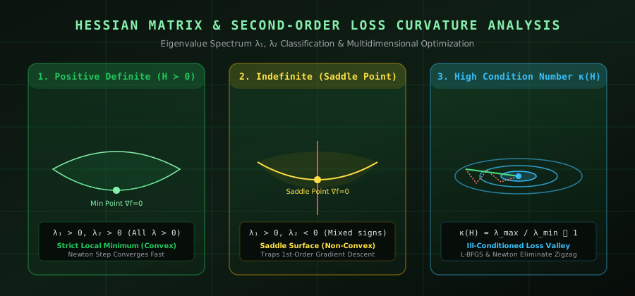
3. Second-Derivative Test in ${\mathbb{R}}^n$ via Eigenvalues

At any stationary critical point ${\mathbf{x}}^{\ast }$ where the gradient vanishes ($\nabla f({\mathbf{x}}^{\ast })=0$), the linear term disappears, and the local topology is governed entirely by the quadratic form $\Delta {\mathbf{x}}^T\mathbf{H}\Delta \mathbf{x}$:

1. Positive Definite ($\mathbf{H}\succ 0$):
   • Condition: $\forall \mathbf{v}\ne 0,{\mathbf{v}}^T\mathbf{Hv}>0⟺{\lambda }_i>0\forall i\in \{1,\dots ,n\}$.
   • Geometry: Strict convex local bowl. ${\mathbf{x}}^{\ast }$ is a strict local minimum.
2. Negative Definite ($\mathbf{H}\prec 0$):
   • Condition: $\forall \mathbf{v}\ne 0,{\mathbf{v}}^T\mathbf{Hv}<0⟺{\lambda }_i<0\forall i\in \{1,\dots ,n\}$.
   • Geometry: Strict concave dome. ${\mathbf{x}}^{\ast }$ is a strict local maximum.
3. Indefinite (Mixed Sign Eigenvalues):
   • Condition: $\exists {\lambda }_i>0$ and $\exists {\lambda }_j<0$.
   • Geometry: Hyperbolic paraboloid. ${\mathbf{x}}^{\ast }$ is a saddle point.
4. Positive / Negative Semi-Definite ($\det (\mathbf{H})=0$, some ${\lambda }_i=0$):
   • Geometry: Degenerate valleys, plateaus, or non-isolated critical lines (further higher-order terms required).

4. The Condition Number $\kappa (\mathbf{H})$ & The Ravine Problem

In gradient descent, the parameter update rule is:

When optimizing a quadratic objective $f(\mathbf{x})=\frac{1}{2}{\mathbf{x}}^T\mathbf{Hx}-{\mathbf{b}}^T\mathbf{x}$, the convergence rate is strictly bounded by the Condition Number of the Hessian:

                ▲ y (High Curvature: λ_max)
                │         /|
                │        / |  (Violent Oscillations)
                │  \    /  |
                │   \  /   |
                │    \/    |
───────────────┼──────────┼──────────────► x (Low Curvature: λ_min)
                │          └─► Slow progress towards optimum

• If $\kappa (\mathbf{H})\approx 1$, the loss contours are spherical hyperspheres, and gradient descent points directly towards the minimum in 1 step.
• If $\kappa (\mathbf{H})\gg 1$ (ill-conditioned loss landscape / ravines):
  • The maximum allowable learning rate is bounded by $\eta <\frac{2}{{\lambda }_{\max }}$ to prevent divergence.
  • The effective convergence rate in the flattest direction is governed by ${\left(\frac{\kappa -1}{\kappa +1}\right)}^2\approx 1-\frac{4}{\kappa }$.
  • This causes gradient descent to zigzag violently across the high-curvature walls while making miniscule progress along the canyon floor.

5. Second-Order Optimization: Newton-Raphson & Quasi-Newton (BFGS / L-BFGS)

Classical Multidimensional Newton-Raphson

To find the step $\Delta \mathbf{x}$ that minimizes the local quadratic Taylor approximation:

Taking the derivative with respect to $\Delta \mathbf{x}$ and setting it to zero:

The Newton-Raphson Update is:

Theoretical Properties:

1. Quadratic Convergence ($\Vert {\mathbf{x}}_{k+1}-{\mathbf{x}}^{\ast }\Vert \le M\Vert {\mathbf{x}}_k-{\mathbf{x}}^{\ast }{\Vert }^2$): Near the minimum, the number of correct decimal digits doubles at each iteration.
2. Curvature Invariance: Newton’s method is affine invariant and eliminates the condition number bottleneck by rescaling the coordinates along principal axes.
3. Computational Bottleneck: Computing $\mathbf{H}$ requires $O(n^2)$ memory and inverting ${\mathbf{H}}^{-1}$ requires $O(n^3)$ operations, rendering pure Newton’s method prohibitive for modern deep neural nets ($n>10^7$).

Quasi-Newton: BFGS & Limited-Memory BFGS (L-BFGS)

Instead of explicitly computing and inverting ${\mathbf{H}}_k$, Quasi-Newton algorithms maintain a running positive-definite approximation ${\mathbf{B}}_k\approx {\mathbf{H}}_k^{-1}$ that satisfies the Secant Equation:

Where ${\mathbf{s}}_k={\mathbf{x}}_{k+1}-{\mathbf{x}}_k$ and ${\mathbf{y}}_k=\nabla f({\mathbf{x}}_{k+1})-\nabla f({\mathbf{x}}_k)$.

The BFGS Inverse Update Formula is given by:

L-BFGS (Limited-Memory BFGS) reduces the memory complexity from $O(n^2)$ to $O(m\cdot n)$ by storing only the most recent $m$ vectors (typically $m\in [5,20]$) and computing the search direction via a two-loop recursion. This is why lbfgs is the gold-standard default solver for Logistic Regression and CRFs in libraries like scikit-learn.

6. The Fisher Information Matrix (FIM) & Natural Gradient Connection

In parametric statistical estimation where the loss is the negative log-likelihood $\mathcal{L}(\theta )=-{\sum }_{i=1}^N\log p({\mathbf{x}}_i|\theta )$, the expected Hessian of the loss is directly equivalent to the Fisher Information Matrix $\mathcal{I}(\theta )$:

Key Statistical Insights:

• Cramér-Rao Lower Bound: For any unbiased estimator $\hat{\theta }$, the covariance matrix is bounded by the inverse Fisher matrix (inverse expected Hessian): $$\mathrm{Cov}(\hat{\theta })⪰\mathcal{I}(\theta {)}^{-1}$$
• Natural Gradient Descent: Amari’s Natural Gradient updates parameters along the Riemannian manifold endowed with the Fisher metric tensor, invariant to parameterization: $${\theta }_{k+1}={\theta }_k-\eta \mathcal{I}({\theta }_k{)}^{-1}\nabla \mathcal{L}({\theta }_k)$$

7. Pearlmutter’s $R$-Operator & Hessian-Vector Products ($\mathbf{Hv}$)

In large-scale deep learning, computing the full $n\times n$ Hessian matrix is impossible. However, second-order solvers like Conjugate Gradient Newton only require the directional derivative of the gradient along a vector $\mathbf{v}$, known as a Hessian-Vector Product (HVP):

Using Pearlmutter’s $R$-operator, reverse-mode automatic differentiation can compute $\mathbf{Hv}$ with the exact same algorithmic time complexity as a single backward pass ($O(n)$)!

8. Practical Implementation in Python & PyTorch

Here is an executable snippet demonstrating how to compute exact Hessians, perform eigenvalue spectrum analysis, and evaluate local loss curvature:

import torch
import numpy as np

# Define a non-linear 2D scalar objective function
def loss_landscape(coords: torch.Tensor) -> torch.Tensor:
    x, y = coords[0], coords[1]
    # Rosenbrock-style non-convex valley
    return 100.0 * (y - x**2)**2 + (1.0 - x)**2

# 1. Compute exact Hessian via PyTorch Autograd
point = torch.tensor([1.2, 0.8], requires_grad=True)
H = torch.autograd.functional.hessian(loss_landscape, point)
grad = torch.autograd.functional.jacobian(loss_landscape, point)

print(f"Gradient at {point.tolist()}:\n{grad.numpy()}\n")
print(f"Hessian Matrix H:\n{H.numpy()}\n")

# 2. Spectral Decomposition of Hessian
eigenvalues, eigenvectors = np.linalg.eigh(H.numpy())
condition_number = np.max(np.abs(eigenvalues)) / np.min(np.abs(eigenvalues))

print(f"Eigenvalues: {eigenvalues}")
print(f"Condition Number κ(H): {condition_number:.2f}")

# 3. Curvature Classification
if np.all(eigenvalues > 0):
    print("=> Region is Strictly Convex (Positive Definite: H ≻ 0)")
elif np.all(eigenvalues < 0):
    print("=> Region is Strictly Concave (Negative Definite: H ≺ 0)")
elif np.any(eigenvalues > 0) and np.any(eigenvalues < 0):
    print("=> Region is a Saddle Point (Indefinite)")

Conclusion & Key Takeaways

1. Gradients dictate direction; Hessians dictate geometry: The Hessian Matrix captures the multi-axis curvature that dictates whether an optimization surface is a bowl, dome, saddle, or narrow ravine.
2. Eigenvalues reveal landscape topology: The signs of $\mathbf{H}$‘s eigenvalues ${\lambda }_i$ classify critical points, while the ratio $\kappa (\mathbf{H})={\lambda }_{\max }/{\lambda }_{\min }$ defines the theoretical limits of first-order convergence.
3. Quasi-Newton & HVPs bridge theory and production: Modern data science exploits L-BFGS, Fisher Information approximations, and $O(n)$ Hessian-Vector Products to harness second-order convergence without incurring the $O(n^3)$ cubic inversion penalty.