Mastering Database Normalization & Analytical Denormalization: From 1NF to BCNF and Modern Lakehouse Star Modeling
An in-depth architectural guide exploring relational normalization forms (1NF, 2NF, 3NF, BCNF) to eliminate modification anomalies, contrasted with analytical denormalization, dimensional star schemas, and modern lakehouse performance optimization.

In database engineering and distributed systems architecture, few concepts have as profound an impact on system throughput, data integrity, and analytical latency as the strategic balance between Relational Normalization and Analytical Denormalization.
While OLTP transactional engines (like PostgreSQL, MySQL, and Oracle) rely on strict mathematical normalization to preserve ACID guarantees and prevent update anomalies, modern distributed analytical warehouses and lakehouses (such as Databricks Delta, Snowflake, and BigQuery) systematically embrace denormalization and wide dimensional modeling to achieve sub-second analytical scans across petabytes of data.
In this deep dive, we will dissect the theoretical mathematics and engineering realities of 1NF through BCNF, investigate the three destructive database anomalies, and master the practical art of dimensional denormalization in enterprise data engineering.
1. The Core Philosophy: Why Do We Normalize?
Normalization is a formal, step-by-step mathematical decomposition of relational tables aimed at achieving two fundamental engineering goals:
- Eliminate Redundant Data Storage: Ensure every discrete atomic fact is stored in exactly one physical location.
- Prevent Database Mutation Anomalies: Ensure that inserting, modifying, or deleting an entity state does not inadvertently corrupt or delete unrelated domain facts.
2. The Three Destructive Anomalies of Unnormalized Data
To understand why normal forms were developed by Edgar F. Codd and Raymond F. Boyce, examine what happens when entity states are coupled inside an unnormalized table:
Consider an unnormalized table: EMPLOYEE_PROJECT_ALLOCATION (EmpID, EmpName, DeptName, DeptManager, ProjectID, ProjectName, AllocationHours).
1. Insertion Anomaly (Inability to record independent facts)
If management creates a new department (e.g., Data Platform Research) with an assigned manager, you cannot insert this department record into the database until at least one employee is hired and assigned to a project, because EmpID or ProjectID forms the primary key.
2. Update Anomaly (Data inconsistency across multiple rows)
If department Enterprise Analytics changes its manager from Alice to Bob, and 5,000 employees work in that department, your application must issue updates across all 5,000 distinct records. If a network interruption or partial failure occurs mid-transaction, the database is left in a corrupted state where some employees report to Alice and others report to Bob.
3. Deletion Anomaly (Unintended collateral data destruction)
If employee John Doe is the only person currently assigned to Project Alpha, and John leaves the company, deleting John’s employee row simultaneously erases all historical existence and metadata of Project Alpha from the enterprise database.
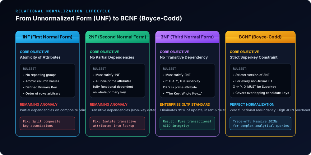
3. The Mathematical Progression: 1NF to BCNF Explained
Let us trace the formal definition and decomposition steps across the normal forms:
First Normal Form (1NF) — Atomicity & Structure
A relation is in 1NF if and only if:
- All column values are atomic (indivisible scalars; no arrays, comma-separated lists, or nested objects).
- There are no repeating groups or multiple columns storing similar items (e.g.,
phone_1,phone_2,phone_3). - Each record is uniquely identifiable by a defined Primary Key.
-- ❌ Violates 1NF (Non-atomic comma-delimited strings)
CREATE TABLE orders_bad (
    order_id INT PRIMARY KEY,
    customer_name VARCHAR(100),
    product_skus VARCHAR(500) -- e.g. 'SKU-01,SKU-09,SKU-44'
);

-- ✅ 1NF Compliant (Decomposed atomic rows)
CREATE TABLE order_items_1nf (
    order_id INT,
    product_sku VARCHAR(50),
    quantity INT,
    PRIMARY KEY (order_id, product_sku)
);
Second Normal Form (2NF) — Removal of Partial Key Dependencies
A relation is in 2NF if:
- It is in 1NF.
- Every non-prime attribute (an attribute not part of any candidate key) is fully functionally dependent on the entire candidate key, rather than on a proper subset of it.
Rule of Thumb: 2NF only applies when a table possesses a composite primary key. If the primary key is a single column, a 1NF table is automatically in 2NF.
-- ❌ Violates 2NF (Composite Key: order_id, product_id)
-- 'product_name' and 'unit_price' depend ONLY on 'product_id', NOT the whole key!
CREATE TABLE order_details_bad (
    order_id INT,
    product_id INT,
    product_name VARCHAR(200), -- Partial dependency!
    unit_price DECIMAL(10,2),  -- Partial dependency!
    quantity_ordered INT,      -- Full dependency on (order_id, product_id)
    PRIMARY KEY (order_id, product_id)
);

-- ✅ 2NF Decomposition: Isolate partial dependencies into PRODUCT table
CREATE TABLE products_2nf (
    product_id INT PRIMARY KEY,
    product_name VARCHAR(200) NOT NULL,
    unit_price DECIMAL(10,2) NOT NULL
);

CREATE TABLE order_items_2nf (
    order_id INT,
    product_id INT REFERENCES products_2nf(product_id),
    quantity_ordered INT NOT NULL,
    PRIMARY KEY (order_id, product_id)
);
Third Normal Form (3NF) — Removal of Transitive Dependencies
A relation is in 3NF if:
- It is in 2NF.
- There are no transitive functional dependencies of non-prime attributes on the primary key ( and , where is the PK and is a non-prime attribute).
Classic Motto (Bill Kent): “Every non-key attribute must provide a fact about the key, the whole key, and nothing but the key, so help me Codd.”
-- ❌ Violates 3NF (Transitive dependency: order_id -> customer_id -> customer_zip -> customer_city)
CREATE TABLE orders_bad_3nf (
    order_id INT PRIMARY KEY,
    order_date DATE,
    customer_id INT,
    customer_zip VARCHAR(10),
    customer_city VARCHAR(100) -- Transitive: customer_zip -> customer_city!
);

-- ✅ 3NF Decomposition: Extract lookup relations
CREATE TABLE zip_codes_3nf (
    zip_code VARCHAR(10) PRIMARY KEY,
    city VARCHAR(100) NOT NULL,
    state VARCHAR(50) NOT NULL
);

CREATE TABLE customers_3nf (
    customer_id INT PRIMARY KEY,
    customer_name VARCHAR(150),
    zip_code VARCHAR(10) REFERENCES zip_codes_3nf(zip_code)
);

CREATE TABLE orders_3nf (
    order_id INT PRIMARY KEY,
    order_date DATE NOT NULL,
    customer_id INT REFERENCES customers_3nf(customer_id)
);
Boyce-Codd Normal Form (BCNF / 3.5NF) — Strict Superkey Rule
A relation is in BCNF if and only if for every non-trivial functional dependency , is a Superkey.
While 3NF permits if is a prime attribute (part of any candidate key), BCNF eliminates this loophole, handling edge cases involving multiple overlapping composite candidate keys.
4. The Analytical Paradigm Shift: Why We Denormalize
While 3NF and BCNF are optimal for single-row OLTP transactions, they create critical performance bottlenecks for analytical queries (OLAP) running over millions or billions of rows.
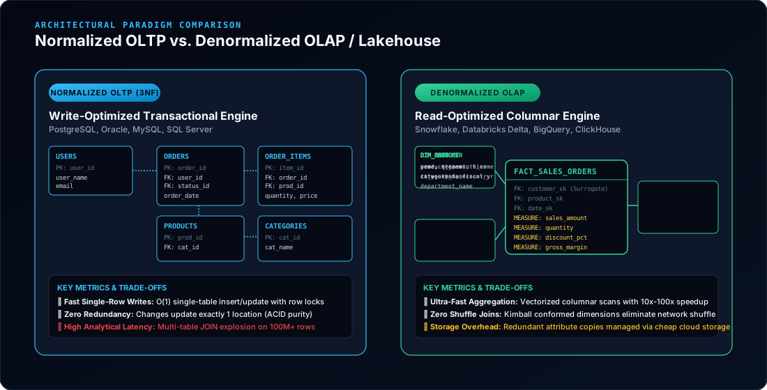
Why 3NF Fails at Scale in Data Warehousing:
- Massive Distributed Shuffle Joins: Joining 8 to 15 normalized tables across a distributed Spark, Snowflake, or Trino cluster forces terabytes of data across physical network switches (hash repartitioning), creating immense I/O latency and memory spill.
- Columnar Inefficiency: Columnar engines (Parquet, ORC, Delta Lake, Snowflake Micro-partitions) compress repetitive column data at ratios of 85%–95%. In a columnar database, duplicate string values in a single wide table cost almost zero additional disk space!
- Query Complexity & BI Tool Bottlenecks: Business analysts and BI tools (Power BI, Tableau) generate simpler, significantly faster SQL when querying a clean Kimball Star Schema or One Big Table (OBT) rather than navigating complex recursive multi-table snowflake graphs.
5. Denormalization Strategies in Modern Data Engineering
Strategy A: The Kimball Dimensional Star Schema
The classic, most resilient approach balances read performance and maintainability:
- Fact Tables: Contain numerical metrics and surrogate keys (
sales_amount,quantity,tax_paid,date_sk,customer_sk). - Conformed Dimension Tables: Denormalize related operational hierarchies (e.g.,
DIM_PRODUCTbundles product, brand, category, subcategory, and supplier into a single wide dimension).
-- High-Performance Denormalized Fact Table Query
SELECT
    d.calendar_year,
    p.category_name,
    c.customer_country,
    SUM(f.sales_amount) AS total_revenue,
    AVG(f.discount_pct) AS avg_discount
FROM FACT_SALES_ORDERS f
JOIN DIM_DATE d ON f.date_sk = d.date_sk
JOIN DIM_PRODUCT p ON f.product_sk = p.product_sk
JOIN DIM_CUSTOMER c ON f.customer_sk = c.customer_sk
WHERE d.calendar_year = 2026
GROUP BY 1, 2, 3
ORDER BY total_revenue DESC;
Strategy B: One Big Table (OBT) in Modern Cloud Warehouses
With modern vectorized query execution (Snowflake Search Optimization, BigQuery Capacitor, Databricks Photon), pre-joining facts and dimensions into a single flattened wide table (OBT_CUSTOMER_ORDERS) completely eliminates runtime JOIN overhead, yielding 5x–20x query speedups on massive dashboards.
Strategy C: Nested & Repeated Structures (Parquet & Delta)
Modern file formats permit semi-structured denormalization (such as ARRAY<STRUCT> in Databricks Spark or BigQuery). This allows maintaining 1-to-many relationships within a single root row without duplicate row multiplication:
-- BigQuery / Spark SQL Nested Denormalization
CREATE TABLE lakehouse_orders (
    order_id STRING,
    order_timestamp TIMESTAMP,
    customer_id STRING,
    total_amount NUMERIC,
    line_items ARRAY<STRUCT<
        product_id STRING,
        item_name STRING,
        unit_price NUMERIC,
        quantity INT64
    >>
);
6. Architecture Comparison & Decision Matrix
| Architectural Dimension | Normalized (3NF / BCNF) | Denormalized (Star Schema / OBT) |
|---|---|---|
| Primary Workload | OLTP (Transactional, CRUD) | OLAP (Analytical, BI, ML) |
| Write Latency | Ultra-Fast (Single localized row updates) | Slower (Batch pipelines, CDC micro-batches) |
| Read Latency (Aggregations) | Slow (Heavy recursive joins) | Sub-Second (Columnar vectorized scans) |
| Data Redundancy | Zero (Pure mathematical single-source) | High (Duplicated dimensional attributes) |
| Storage Cost Sensitivity | Minimal storage footprint | Slightly higher raw size (mitigated by compression) |
| Integrity Enforcement | RDBMS Foreign Keys & Constraints | Upstream ETL/ELT rules (dbt tests, CDQ) |
| Ideal Compute Engines | PostgreSQL, MySQL, Spanner, Oracle | Databricks Delta, Snowflake, BigQuery, ClickHouse |
7. The Hybrid Lakehouse Architecture: Best of Both Worlds
In production enterprise platforms, the industry has standardized on a hybrid continuum:
- Operational Layer (OLTP): Application databases are normalized to 3NF to handle thousands of concurrent sub-millisecond ACID transactions with zero locking anomalies.
- Bronze / Silver Lakehouse Layer: Change Data Capture (CDC) streams transactions into a normalized or conformed Silver Delta/Iceberg layer, applying SCD Type 2 history tracking.
- Gold Mart Layer: Scheduled ELT transformations (dbt / Spark) denormalize Silver tables into optimized Star Schemas and One Big Tables (OBT) tailored for executive dashboards and real-time ad-hoc analytics.
By understanding the mathematical constraints of 1NF–BCNF alongside the hardware and distributed dynamics of columnar compute, data architects can deliver both uncompromised transactional safety and blazingly fast analytical throughput.
Rahul Das
Senior Data EngineerBuilding resilient streaming pipelines, cloud lakehouses, and high-performance data architectures. Let's connect!